Exploratory Data Analysis

# Basic System & Math Utilities
import os
import math
import glob

# Audio Processing Libraries
import wave
import librosa
import librosa.display
import soundfile
from scipy.io.wavfile import read

# Data Handling & Numerical Computing
import numpy as np
import pandas as pd
from scipy.stats import chi2_contingency
from scipy.stats import f_oneway

# Visualization Tools
import matplotlib.pyplot as plt
import seaborn as sns

%matplotlib inline

# Machine Learning / Deep Learning
import tensorflow as tf
from tqdm.notebook import tqdm

# Jupyter Audio Playback
import IPython.display as ipd

from tqdm.notebook import tqdm

Explore Dataset Directory

import kagglehub
vbookshelf_respiratory_sound_database_path = kagglehub.dataset_download('vbookshelf/respiratory-sound-database')

print('Data source import complete.')

Downloading from https://www.kaggle.com/api/v1/datasets/download/vbookshelf/respiratory-sound-database?dataset_version_number=2...

100%|██████████| 3.69G/3.69G [00:41<00:00, 95.2MB/s]

Extracting files...

Data source import complete.

The dataset used in this study is the Respiratory Sound Database, originally acquired from the Biomedical Health Informatics Challenge hosted by Aristotle University of Thessaloniki (Rocha et al., 2019). This database was curated by research teams from Portugal and Greece and is publicly accessible via Kaggle.

The dataset comprises 920 annotated audio recordings of respiratory sounds from 126 patients, with clips ranging from 10 to 90 seconds in length. Each recording includes corresponding annotation files that describe the presence of respiratory anomalies such as wheezes, crackles, or both, as well as demographic and diagnostic information for each patient. The dataset offers a comprehensive repository of real-world respiratory sound data, suitable for training and evaluating machine learning models targeting respiratory disease detection.

os.listdir(vbookshelf_respiratory_sound_database_path)

['respiratory_sound_database',
 'Respiratory_Sound_Database',
 'demographic_info.txt']

Load and Merge Demographics & Diagnosis CSVs

df_no_diagnosis = pd.read_csv(
    os.path.join(vbookshelf_respiratory_sound_database_path, 'demographic_info.txt'),
    names=['Patient number', 'Age', 'Sex', 'Adult BMI (kg/m2)',
           'Child Weight (kg)', 'Child Height (cm)'],
    delimiter=' '
)

diagnosis = pd.read_csv(
    os.path.join(vbookshelf_respiratory_sound_database_path, 'Respiratory_Sound_Database',
                 'Respiratory_Sound_Database', 'patient_diagnosis.csv'),
    names=['Patient number', 'Diagnosis']
)

# Merge demographics + diagnosis
df = df_no_diagnosis.join(
    diagnosis.set_index('Patient number'),
    on='Patient number',
    how='left'
)

df

	Patient number	Age	Sex	Adult BMI (kg/m2)	Child Weight (kg)	Child Height (cm)	Diagnosis
0	101	3.00	F	NaN	19.0	99.0	URTI
1	102	0.75	F	NaN	9.8	73.0	Healthy
2	103	70.00	F	33.00	NaN	NaN	Asthma
3	104	70.00	F	28.47	NaN	NaN	COPD
4	105	7.00	F	NaN	32.0	135.0	URTI
...	...	...	...	...	...	...	...
121	222	60.00	M	NaN	NaN	NaN	COPD
122	223	NaN	NaN	NaN	NaN	NaN	COPD
123	224	10.00	F	NaN	32.3	143.0	Healthy
124	225	0.83	M	NaN	7.8	74.0	Healthy
125	226	4.00	M	NaN	16.7	103.0	Pneumonia

126 rows × 7 columns

List All Filenames

root = os.path.join(vbookshelf_respiratory_sound_database_path, 'Respiratory_Sound_Database', 'Respiratory_Sound_Database', 'audio_and_txt_files') + os.sep

filenames = [s.split('.')[0] for s in os.listdir(root) if s.endswith('.txt')]

Function to Extract Annotation Data

def Extract_Annotation_Data(file_name, root):
    tokens = file_name.split('_')

    recording_info = pd.DataFrame(
        data=[tokens],
        columns=['Patient number', 'Recording index',
                 'Chest location', 'Acquisition mode', 'Recording equipment']
    )

    recording_annotations = pd.read_csv(
        os.path.join(root, file_name + '.txt'),
        names=['Start', 'End', 'Crackles', 'Wheezes'],
        delimiter='\t'
    )

    return recording_info, recording_annotations

Collect Recording Info & Annotation Dictionaries

i_list = []
rec_annotations_dict = {}

for s in filenames:
    info, ann = Extract_Annotation_Data(s, root)
    i_list.append(info)
    rec_annotations_dict[s] = ann

recording_info = pd.concat(i_list, axis=0)
recording_info.tail()

	Patient number	Recording index	Chest location	Acquisition mode	Recording equipment
0	205	1b3	Al	mc	AKGC417L
0	166	1p1	Pl	sc	Meditron
0	109	1b1	Al	sc	Litt3200
0	108	1b1	Al	sc	Meditron
0	159	1b1	Al	sc	Meditron

Count Crackles/Wheezes Per File

filename_list = []
no_label_list = []
crack_list = []
wheeze_list = []
both_sym_list = []

for f in filenames:
    d = rec_annotations_dict[f]

    no_label = len(d[(d['Crackles'] == 0) & (d['Wheezes'] == 0)])
    crack_only = len(d[(d['Crackles'] == 1) & (d['Wheezes'] == 0)])
    wheeze_only = len(d[(d['Crackles'] == 0) & (d['Wheezes'] == 1)])
    both = len(d[(d['Crackles'] == 1) & (d['Wheezes'] == 1)])

    filename_list.append(f)
    no_label_list.append(no_label)
    crack_list.append(crack_only)
    wheeze_list.append(wheeze_only)
    both_sym_list.append(both)

file_label_df = pd.DataFrame({
    'filename': filename_list,
    'no label': no_label_list,
    'crackles only': crack_list,
    'wheezes only': wheeze_list,
    'crackles and wheezees': both_sym_list
})

Aggregate & Assign Diagnosis Labels

labels = file_label_df.sort_values(by='filename')
summary = labels.groupby('filename').sum()

conditions = [
    (summary['crackles only'] == 0) &
    (summary['wheezes only'] == 0) &
    (summary['crackles and wheezees'] == 0),

    (summary['crackles only'] == summary.max(axis=1)),
    (summary['wheezes only'] == summary.max(axis=1)),
    (summary['crackles and wheezees'] == summary.max(axis=1)),

    (summary['no label'] == summary.max(axis=1)) &
    (summary['crackles only'] > summary['wheezes only']) &
    (summary['crackles only'] > summary['crackles and wheezees']),

    (summary['no label'] == summary.max(axis=1)) &
    (summary['wheezes only'] >= summary['crackles only']) &
    (summary['wheezes only'] > summary['crackles and wheezees']),

    (summary['no label'] == summary.max(axis=1)) &
    (summary['crackles and wheezees'] >= summary['crackles only']) &
    (summary['crackles and wheezees'] >= summary['wheezes only']),
]

values = [
    'Healthy',
    'Crackles',
    'Wheezes',
    'Wheezes & Crackles',
    'Crackles',
    'Wheezes',
    'Wheezes & Crackles'
]

summary['diagnosis'] = np.select(conditions, values, default='Unknown')
summary

	no label	crackles only	wheezes only	crackles and wheezees	diagnosis
filename
101_1b1_Al_sc_Meditron	12	0	0	0	Healthy
101_1b1_Pr_sc_Meditron	11	0	0	0	Healthy
102_1b1_Ar_sc_Meditron	13	0	0	0	Healthy
103_2b2_Ar_mc_LittC2SE	2	0	4	0	Wheezes
104_1b1_Al_sc_Litt3200	6	0	0	0	Healthy
...	...	...	...	...	...
224_1b2_Al_sc_Meditron	7	0	0	0	Healthy
225_1b1_Pl_sc_Meditron	14	0	0	0	Healthy
226_1b1_Al_sc_Meditron	8	2	0	0	Crackles
226_1b1_Ll_sc_Meditron	4	6	0	0	Crackles
226_1b1_Pl_sc_LittC2SE	6	5	0	0	Crackles

920 rows × 5 columns

Exploratory Data Analysis

Basic Overview of Demographic Dataset

print("Shape of demographics dataframe:", df.shape)
df.head()

Shape of demographics dataframe: (126, 7)

	Patient number	Age	Sex	Adult BMI (kg/m2)	Child Weight (kg)	Child Height (cm)	Diagnosis
0	101	3.00	F	NaN	19.0	99.0	URTI
1	102	0.75	F	NaN	9.8	73.0	Healthy
2	103	70.00	F	33.00	NaN	NaN	Asthma
3	104	70.00	F	28.47	NaN	NaN	COPD
4	105	7.00	F	NaN	32.0	135.0	URTI

# Check missing values
df.isnull().sum()

	0
Patient number	0
Age	1
Sex	1
Adult BMI (kg/m2)	51
Child Weight (kg)	82
Child Height (cm)	84
Diagnosis	0

dtype: int64

# Summary statistics
df.describe(include='all')

	Patient number	Age	Sex	Adult BMI (kg/m2)	Child Weight (kg)	Child Height (cm)	Diagnosis
count	126.000000	125.00000	125	75.000000	44.000000	42.000000	126
unique	NaN	NaN	2	NaN	NaN	NaN	8
top	NaN	NaN	M	NaN	NaN	NaN	COPD
freq	NaN	NaN	79	NaN	NaN	NaN	64
mean	163.500000	42.99264	NaN	27.190000	21.361136	104.652381	NaN
std	36.517119	32.20907	NaN	5.372519	17.150885	30.793128	NaN
min	101.000000	0.25000	NaN	16.500000	7.140000	64.000000	NaN
25%	132.250000	4.00000	NaN	24.150000	11.755000	81.250000	NaN
50%	163.500000	60.00000	NaN	27.400000	15.100000	99.500000	NaN
75%	194.750000	71.00000	NaN	29.185000	24.325000	117.750000	NaN
max	226.000000	93.00000	NaN	53.500000	80.000000	183.000000	NaN

Diagnosis Distribution

plt.figure(figsize=(8,5))
sns.countplot(data=df, x='Diagnosis')
plt.title("Distribution of Patient Diagnoses")
plt.xticks(rotation=45)
plt.show()

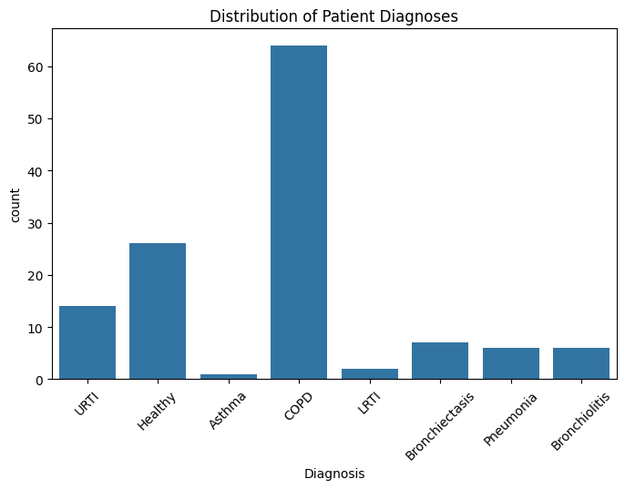
This bar chart shows the distribution of patient diagnoses in the dataset by count.

Dominant and Minority Classes

• COPD (Chronic Obstructive Pulmonary Disease) is the most represented diagnosis by far, with over 60 patients, making it the majority class in this sample.

• Healthy individuals form the second largest group, with just over 25 cases, providing a sizeable control population for comparative analysis.

• URTI (Upper Respiratory Tract Infection) is also notable, but substantially fewer than COPD and Healthy, with around 15 cases.

• Diagnoses like Asthma, LRTI (Lower Respiratory Tract Infection), Bronchiectasis, Pneumonia, and Bronchiolitis are minority classes, each with less than 10 cases, indicating limited sampling or rarity in the dataset.

Analytical Implications

• The diagnosis distribution is highly imbalanced, especially with the dominance of COPD and the scarcity of less common conditions.

• Models trained on this dataset may require strategies to handle class imbalance, such as oversampling minority classes, using class weights, or designing specific evaluation metrics to prevent bias toward COPD detection.

• The strong representation of Healthy and COPD is beneficial for discriminative modeling but highlights the risk of reduced sensitivity and lower generalizability for rare diseases (e.g., Asthma, Bronchiolitis).

Epidemiological Considerations

• High COPD counts may reflect real-world prevalence patterns, especially in older, smoking, or at-risk populations, or could be due to targeted recruitment in the dataset.

• The rarity of asthma and select infections could indicate these conditions are less prevalent in the sampled cohort or might result from inclusion criteria and annotation emphasis.

plt.figure(figsize=(7,5))
sns.countplot(data=df, x='Sex', hue='Diagnosis')
plt.title("Gender vs Diagnosis")
plt.show()

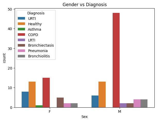
This grouped bar chart displays counts of recordings by diagnosis and sex (female “F” and male “M”) for several respiratory conditions.

Major Trends

• COPD (Chronic Obstructive Pulmonary Disease) shows a strong male predominance, with more than triple the number of male cases compared to females.

• Healthy individuals are distributed equally between sexes, suggesting the reference population is balanced.

• URTI (Upper Respiratory Tract Infection), Bronchiectasis, Pneumonia, and Bronchiolitis have lower and fairly balanced counts across both sexes, indicating no strong gender bias in sample collection for these conditions.

Observations

• Asthma is notably rare in this subset, with only 1 female case and none in males—highlighting potential sampling or annotation limitations for this diagnosis.

• LRTI (Lower Respiratory Tract Infection) is more frequent in males but remains one of the less common classes overall.

Overview of Audio-Based Labels

labels_df_recreated = file_label_df.sort_values(by='filename')
summary = labels_df_recreated.groupby('filename').sum()

# Re-apply the logic
conditions = [
    (summary['crackles only'] == 0) &
    (summary['wheezes only'] == 0) &
    (summary['crackles and wheezees'] == 0),

    (summary['crackles only'] == summary.max(axis=1)),
    (summary['wheezes only'] == summary.max(axis=1)),
    (summary['crackles and wheezees'] == summary.max(axis=1)),

    (summary['no label'] == summary.max(axis=1)) &
    (summary['crackles only'] > summary['wheezes only']) &
    (summary['crackles only'] > summary['crackles and wheezees']),

    (summary['no label'] == summary.max(axis=1)) &
    (summary['wheezes only'] >= summary['crackles only']) &
    (summary['wheezes only'] > summary['crackles and wheezees']),

    (summary['no label'] == summary.max(axis=1)) &
    (summary['crackles and wheezees'] >= summary['crackles only']) &
    (summary['crackles and wheezees'] >= summary['wheezes only']),
]

values = [
    'Healthy',
    'Crackles',
    'Wheezes',
    'Wheezes & Crackles',
    'Crackles',
    'Wheezes',
    'Wheezes & Crackles'
]

summary['diagnosis'] = np.select(conditions, values, default='Unknown')

# Reset the index to make 'filename' a regular column, which is often easier for merging.
# This ensures the actual filenames are in a column named 'filename'.
summary = summary.reset_index().rename(columns={'index': 'filename'})

# Ensure the 'filename' column is explicitly string type to use .str accessor reliably
summary['filename'] = summary['filename'].astype(str)

# Extract Patient number from the 'filename' column
# The filename format is 'PATIENT_NUMBER_RECORDING_INDEX_...'
summary['Patient number'] = summary['filename'].str.split('_').str[0].astype(int)

# Rename the existing audio-based diagnosis column before merging to avoid name collision
summary = summary.rename(columns={'diagnosis': 'audio_diagnosis'})

# Merge with the main demographic and diagnosis DataFrame (df)
# Select only the 'Patient number' and 'Diagnosis' columns from df
# Assuming 'df' is available from previous cells
df_patient_diagnosis = df[['Patient number', 'Diagnosis']].drop_duplicates(subset=['Patient number'])

# Perform the merge. The clinical diagnosis column will be named 'Diagnosis'.
summary = pd.merge(summary, df_patient_diagnosis, on='Patient number', how='left')

# Rename the merged clinical 'Diagnosis' column for clarity
summary = summary.rename(columns={'Diagnosis': 'clinical_diagnosis'})

summary.head()

	filename	no label	crackles only	wheezes only	crackles and wheezees	audio_diagnosis	Patient number	clinical_diagnosis
0	101_1b1_Al_sc_Meditron	12	0	0	0	Healthy	101	URTI
1	101_1b1_Pr_sc_Meditron	11	0	0	0	Healthy	101	URTI
2	102_1b1_Ar_sc_Meditron	13	0	0	0	Healthy	102	Healthy
3	103_2b2_Ar_mc_LittC2SE	2	0	4	0	Wheezes	103	Asthma
4	104_1b1_Al_sc_Litt3200	6	0	0	0	Healthy	104	COPD

Overview of Audio VS Demographic Datasets

columns_to_check = ['Age', 'Sex', 'Diagnosis', 'audio_diagnosis']

# Extract 'Patient number' from the 'filename' column of the 'summary' DataFrame
summary_with_patient_id = summary.copy()
summary_with_patient_id['Patient number'] = summary_with_patient_id['filename'].str.split('_').str[0].astype(int)

# Merge df (demographic/clinical diagnosis) with summary (audio-based diagnosis)
# Only select the patient number and the audio-based diagnosis from summary_with_patient_id
merged_data = df.merge(summary_with_patient_id[['Patient number', 'audio_diagnosis']], on='Patient number', how='inner')

cleaned_merged_data = merged_data.dropna(subset=columns_to_check).copy()

print(f"Original merged_data shape: {merged_data.shape}")
print(f"Cleaned merged_data shape: {cleaned_merged_data.shape}")

print("First 5 rows of cleaned_merged_data:")
cleaned_merged_data.head()

Original merged_data shape: (920, 8)
Cleaned merged_data shape: (914, 8)
First 5 rows of cleaned_merged_data:

	Patient number	Age	Sex	Adult BMI (kg/m2)	Child Weight (kg)	Child Height (cm)	Diagnosis	audio_diagnosis
0	101	3.00	F	NaN	19.0	99.0	URTI	Healthy
1	101	3.00	F	NaN	19.0	99.0	URTI	Healthy
2	102	0.75	F	NaN	9.8	73.0	Healthy	Healthy
3	103	70.00	F	33.00	NaN	NaN	Asthma	Wheezes
4	104	70.00	F	28.47	NaN	NaN	COPD	Healthy

##Analyze Age vs. Respiratory Sound Patterns (ANOVA)

# Get unique values from the 'diagnosis' column
relevant_audio_diagnoses = cleaned_merged_data['audio_diagnosis'].unique()

# Create a list of age arrays for each audio-based diagnosis group
age_groups_audio = [cleaned_merged_data['Age'][cleaned_merged_data['audio_diagnosis'] == d].dropna() for d in relevant_audio_diagnoses]

# Perform one-way ANOVA test
f_statistic_audio, p_value_audio = f_oneway(*age_groups_audio)

# Calculate degrees of freedom
df_between_audio = len(relevant_audio_diagnoses) - 1
df_within_audio = sum(len(group) for group in age_groups_audio) - len(relevant_audio_diagnoses)

# Calculate eta-squared (η²) and eta (η)
eta_squared_audio = (f_statistic_audio * df_between_audio) / (f_statistic_audio * df_between_audio + df_within_audio)
eta_age_audio = np.sqrt(eta_squared_audio)

print(f"One-way ANOVA for Age vs. Respiratory Sound Patterns:")
print(f"F-statistic: {f_statistic_audio:.3f}")
print(f"P-value: {p_value_audio:.3f}")
print(f"Correlation Ratio (η) for Age vs. Respiratory Sound Patterns: {eta_age_audio:.3f}")

One-way ANOVA for Age vs. Respiratory Sound Patterns:
F-statistic: 17.229
P-value: 0.000
Correlation Ratio (η) for Age vs. Respiratory Sound Patterns: 0.232

One-way ANOVA shows a statistically significant difference in mean age across audio-based diagnosis groups (F(2, N−3) = 17.23, p < 0.001). However, the correlation ratio (η = 0.232; η² ≈ 0.054) indicates a small effect — only ~5.4% of age variance is explained by diagnosis group. Clinically, older participants appear slightly more likely to have crackles or mixed findings, but age alone is a weak predictor of respiratory sound class and should not be used as a surrogate for diagnostic category.

Analyze Gender vs. Respiratory Sound Patterns (Chi-squared)

# 1. Create a contingency table
contingency_table_audio = pd.crosstab(cleaned_merged_data['Sex'], cleaned_merged_data['audio_diagnosis'])

# 3. Perform the Chi-squared test of independence
chi2_audio, p_audio, dof_audio, expected_audio = chi2_contingency(contingency_table_audio)

# 4. Print the chi-squared statistic and the p-value
print(f"Chi-squared statistic for Gender vs. Respiratory Sound Patterns: {chi2_audio:.3f}")
print(f"P-value for Gender vs. Respiratory Sound Patterns: {p_audio:.3f}")

Chi-squared statistic for Gender vs. Respiratory Sound Patterns: 25.522
P-value for Gender vs. Respiratory Sound Patterns: 0.000

def calculate_cramers_v(contingency_table, chi2):
    n = contingency_table.sum().sum()
    min_dim = min(contingency_table.shape)
    v = np.sqrt(chi2 / (n * (min_dim - 1)))
    return v

cramers_v_audio = calculate_cramers_v(contingency_table_audio, chi2_audio)
print(f"Cramers V for Gender vs. Respiratory Sound Patterns: {cramers_v_audio:.3f}")

Cramers V for Gender vs. Respiratory Sound Patterns: 0.167

The Chi-squared test showed a statistically significant association between gender and audio-based diagnosis (χ² = 25.52, p < 0.001). However, the effect size was small (Cramer’s V = 0.167), indicating that gender has only a weak relationship with the presence of crackles, wheezes, or combined sounds. Gender should therefore not be considered a strong predictor of respiratory sound category.

Analyze Age vs. Clinical Diagnosis (ANOVA)

# 1. Get unique values from the 'Diagnosis' column
demographic_diagnoses = cleaned_merged_data['Diagnosis'].unique()

# 2. Create a list of age arrays for each demographic diagnosis group
age_groups_demographic = [cleaned_merged_data['Age'][cleaned_merged_data['Diagnosis'] == d].dropna() for d in demographic_diagnoses]

# 3. Perform one-way ANOVA test
f_statistic_demographic, p_value_demographic = f_oneway(*age_groups_demographic)

# Calculate degrees of freedom
df_between_demographic = len(demographic_diagnoses) - 1
df_within_demographic = sum(len(group) for group in age_groups_demographic) - len(demographic_diagnoses)

# Calculate eta-squared (η²) and eta (η)
eta_squared_demographic = (f_statistic_demographic * df_between_demographic) / (f_statistic_demographic * df_between_demographic + df_within_demographic)
eta_age_demographic = np.sqrt(eta_squared_demographic)

# 4. Print the F-statistic and p-value
print(f"One-way ANOVA for Age vs. Clinical Diagnoses:")
print(f"F-statistic: {f_statistic_demographic:.3f}")
print(f"P-value: {p_value_demographic:.3f}")
print(f"Correlation Ratio (η) for Age vs. Clinical Diagnoses: {eta_age_demographic:.3f}")

One-way ANOVA for Age vs. Clinical Diagnoses:
F-statistic: 418.525
P-value: 0.000
Correlation Ratio (η) for Age vs. Clinical Diagnoses: 0.874

One-way ANOVA revealed a highly significant difference in age across demographic diagnosis groups (F = 418.53, p < 0.001). The correlation ratio was very large(η = 0.874, η² ≈ 0.763), indicating that diagnosis category strongly depends on age. Approximately 76% of the variance in age is explained by diagnostic group assignment, reflecting the well-known age-related distribution of diseases such as COPD (older adults) versus asthma (younger individuals).

Analyze Gender vs. Clinical Diagnosis (Chi-squared)

# 1. Create a contingency table
contingency_table_demographic = pd.crosstab(cleaned_merged_data['Sex'], cleaned_merged_data['Diagnosis'])

# 2. Perform the Chi-squared test of independence
chi2_demographic, p_demographic, dof_demographic, expected_demographic = chi2_contingency(contingency_table_demographic)

# 3. Print the chi-squared statistic and the p-value
print(f"Chi-squared statistic for Gender vs. Clinical Diagnoses: {chi2_demographic:.3f}")
print(f"P-value for Gender vs. Clinical Diagnoses: {p_demographic:.3f}")

Chi-squared statistic for Gender vs. Clinical Diagnoses: 31.036
P-value for Gender vs. Clinical Diagnoses: 0.000

cramers_v_demographic = calculate_cramers_v(contingency_table_demographic, chi2_demographic)
print(f"Cramers V for Gender vs. Clinical Diagnoses: {cramers_v_demographic:.3f}")

Cramers V for Gender vs. Clinical Diagnoses: 0.184

This shows a statistically significant association between gender and respiratory diagnoses (p = 0.000), indicating that certain conditions are more common in one gender than the other. However, the strength of this association is weak to moderate (Cramér’s V = 0.184), meaning gender alone is not a strong predictor of diagnosis. Clinically, while slight gender trends may exist, gender should be considered alongside other features for accurate assessment or modeling.

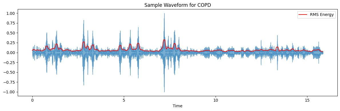
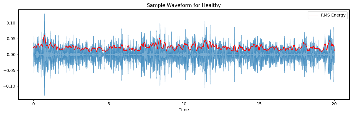
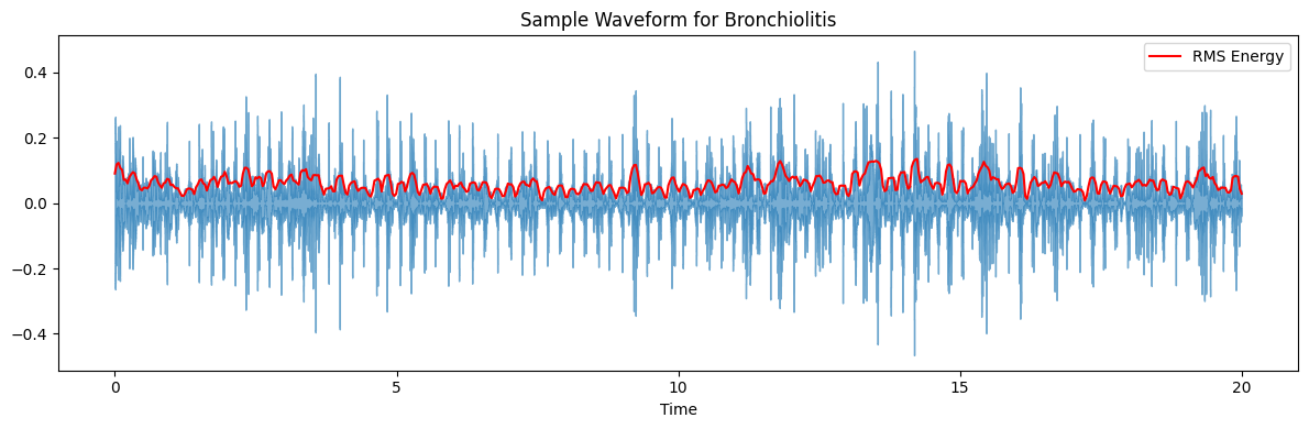
Example Waveform and Spectrogram Visual

i = 100
sound_filename = root + file_label_df['filename'][i] + '.wav'

ipd.Audio(sound_filename, rate=16000)

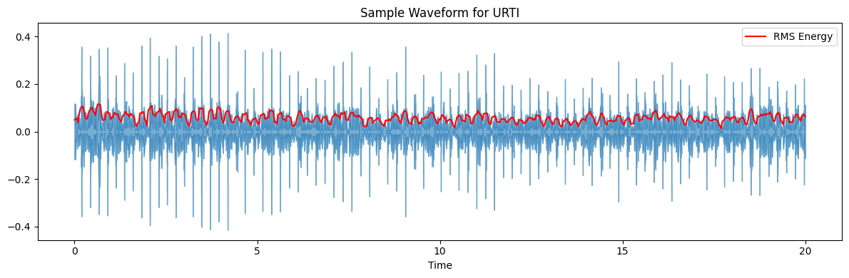
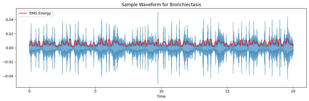
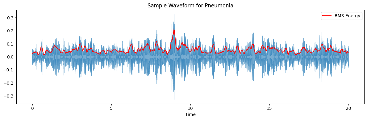
target_diagnoses = ['COPD', 'Healthy', 'URTI', 'Bronchiectasis', 'Pneumonia', 'Bronchiolitis']

# Define hop_length explicitly so both RMS and Time calculation use the same value
hop_length = 512

for diagnosis_type in target_diagnoses:
    # Find the first filename for the current diagnosis type
    # Note: Ensure 'summary' dataframe and 'root' path are defined in your environment
    # The 'filename' column must be present in the 'summary' DataFrame after jo2rAMCoOT09 is run correctly.
    example_filename = summary[summary['clinical_diagnosis'] == diagnosis_type]['filename'].iloc[0]

    # Construct the full path to the WAV file
    wav_path = os.path.join(root, example_filename + '.wav')

    # Load the audio file
    x, sr = librosa.load(wav_path, sr=16000)

    # Calculate RMS energy
    # Explicitly passing hop_length ensures consistency
    rms = librosa.feature.rms(y=x, hop_length=hop_length)

    # We must tell times_like what the SR and hop_length are
    times = librosa.times_like(rms, sr=sr, hop_length=hop_length)

    # Create a figure and axes for plotting
    plt.figure(figsize=(12, 4))
    ax = plt.subplot(1, 1, 1)

    # Plot the waveform
    librosa.display.waveshow(y=x, sr=sr, ax=ax, alpha=0.6)

    # Overlay the RMS envelope
    ax.plot(times, rms[0], color='r', linestyle='-', label='RMS Energy')
    ax.legend()

    # Set plot title
    ax.set(title=f'Sample Waveform for {diagnosis_type}')
    plt.tight_layout()
    plt.show()

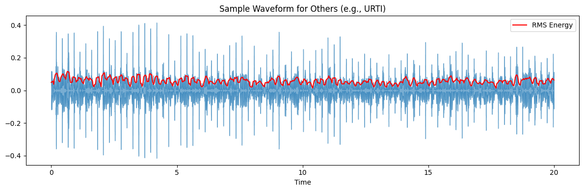
target_plot_categories = ['COPD', 'Healthy', 'Pneumonia', 'Others']

hop_length = 512

for category_type in target_plot_categories:
    if category_type == 'Others':
        # Select one diagnosis from the 'Others' group to represent it
        # 'URTI' is chosen as a representative example from the 'Others' group
        example_diagnosis_for_others = 'URTI'
        example_filename = summary[summary['clinical_diagnosis'] == example_diagnosis_for_others]['filename'].iloc[0]
        plot_title_diagnosis = f'Sample Waveform for {category_type} (e.g., {example_diagnosis_for_others})'
    else:
        example_filename = summary[summary['clinical_diagnosis'] == category_type]['filename'].iloc[0]
        plot_title_diagnosis = f'Sample Waveform for {category_type}'

    # Construct the full path to the WAV file
    wav_path = os.path.join(root, example_filename + '.wav')

    # Load the audio file
    x, sr = librosa.load(wav_path, sr=16000)

    # Calculate RMS energy
    rms = librosa.feature.rms(y=x, hop_length=hop_length)

    # Define times for RMS envelope
    times = librosa.times_like(rms, sr=sr, hop_length=hop_length)

    # Create a figure and axes for plotting
    plt.figure(figsize=(12, 4))
    ax = plt.subplot(1, 1, 1)

    # Plot the waveform
    librosa.display.waveshow(y=x, sr=sr, ax=ax, alpha=0.6)

    # Overlay the RMS envelope
    ax.plot(times, rms[0], color='r', linestyle='-', label='RMS Energy')
    ax.legend()

    # Set plot title
    ax.set(title=plot_title_diagnosis)
    plt.tight_layout()
    plt.show()

Extract Audio Features

# 1. Re-create summary DataFrame with clinical diagnosis to ensure data consistency
labels_df_recreated = file_label_df.sort_values(by='filename')
summary_temp = labels_df_recreated.groupby('filename').sum()

conditions = [
    (summary_temp['crackles only'] == 0) &
    (summary_temp['wheezes only'] == 0) &
    (summary_temp['crackles and wheezees'] == 0),

    (summary_temp['crackles only'] == summary_temp.max(axis=1)),
    (summary_temp['wheezes only'] == summary_temp.max(axis=1)),
    (summary_temp['crackles and wheezees'] == summary_temp.max(axis=1)),

    (summary_temp['no label'] == summary_temp.max(axis=1)) &
    (summary_temp['crackles only'] > summary_temp['wheezes only']) &
    (summary_temp['crackles only'] > summary_temp['crackles and wheezees']),

    (summary_temp['no label'] == summary_temp.max(axis=1)) &
    (summary_temp['wheezes only'] >= summary_temp['crackles only']) &
    (summary_temp['wheezes only'] > summary_temp['crackles and wheezees']),

    (summary_temp['no label'] == summary_temp.max(axis=1)) &
    (summary_temp['crackles and wheezees'] >= summary_temp['crackles only']) &
    (summary_temp['crackles and wheezees'] >= summary_temp['wheezes only']),
]

values = [
    'Healthy',
    'Crackles',
    'Wheezes',
    'Wheezes & Crackles',
    'Crackles',
    'Wheezes',
    'Wheezes & Crackles'
]

summary_temp['diagnosis'] = np.select(conditions, values, default='Unknown')

# Reset the index to make 'filename' a regular column
summary_merged = summary_temp.reset_index().rename(columns={'index': 'filename'})

# Ensure the 'filename' column is explicitly string type
summary_merged['filename'] = summary_merged['filename'].astype(str)

# Extract Patient number from the 'filename' column
summary_merged['Patient number'] = summary_merged['filename'].str.split('_').str[0].astype(int)

# Rename the existing audio-based diagnosis column
summary_merged = summary_merged.rename(columns={'diagnosis': 'audio_diagnosis'})

# Merge with the main demographic and diagnosis DataFrame (df)
df_patient_diagnosis = df[['Patient number', 'Diagnosis']].drop_duplicates(subset=['Patient number'])
summary_merged = pd.merge(summary_merged, df_patient_diagnosis, on='Patient number', how='left')

# Rename the merged clinical 'Diagnosis' column for clarity
summary_merged = summary_merged.rename(columns={'Diagnosis': 'clinical_diagnosis'})

print("Recreated summary_merged DataFrame with clinical diagnosis.")

# 2. & 3. Extract Audio Features and create features_df
all_audio_features = []
sr_new = 16000 # Standardize sample rate to 16kHz for feature extraction

for index, row in tqdm(summary_merged.iterrows(), total=summary_merged.shape[0], desc="Extracting Audio Features"):
    filename = row['filename']
    clinical_diagnosis = row['clinical_diagnosis']
    audio_diagnosis = row['audio_diagnosis']

    wav_path = os.path.join(root, filename + '.wav')

    try:
        y, sr_original = librosa.load(wav_path, sr=None) # Load with original sample rate

        # Resample if original sample rate is different from target
        if sr_original != sr_new:
            y_resampled = librosa.resample(y=y, orig_sr=sr_original, target_sr=sr_new)
        else:
            y_resampled = y

        # Calculate duration
        duration = len(y_resampled) / sr_new # Use resampled length and new SR

        # Calculate Spectral Centroid
        spectral_centroid = np.mean(librosa.feature.spectral_centroid(y=y_resampled, sr=sr_new))

        # Calculate Spectral Bandwidth
        spectral_bandwidth = np.mean(librosa.feature.spectral_bandwidth(y=y_resampled, sr=sr_new))

        # Calculate Spectral Roll-off
        spectral_rolloff = np.mean(librosa.feature.spectral_rolloff(y=y_resampled, sr=sr_new))

        # Calculate Spectral Flux using onset_strength as a proxy
        onset_env = librosa.onset.onset_strength(y=y_resampled, sr=sr_new)
        spectral_flux = np.mean(onset_env)

        all_audio_features.append({
            'filename': filename,
            'clinical_diagnosis': clinical_diagnosis,
            'audio_diagnosis': audio_diagnosis,
            'original_sample_rate': sr_original,
            'duration_sec': duration,
            'spectral_centroid': spectral_centroid,
            'spectral_bandwidth': spectral_bandwidth,
            'spectral_rolloff': spectral_rolloff,
            'spectral_flux': spectral_flux
        })

    except Exception as e:
        print(f"Error processing {filename}: {e}")
        all_audio_features.append({
            'filename': filename,
            'clinical_diagnosis': clinical_diagnosis,
            'audio_diagnosis': audio_diagnosis,
            'original_sample_rate': None,
            'duration_sec': None,
            'spectral_centroid': None,
            'spectral_bandwidth': None,
            'spectral_rolloff': None,
            'spectral_flux': None
        })

features_df = pd.DataFrame(all_audio_features)
print("Audio feature extraction complete.")

# 4. Group by clinical_diagnosis and aggregate, creating a new 'grouped_clinical_diagnosis'
def group_diagnoses_for_mean_features(diagnosis):
    if diagnosis in ['Healthy', 'COPD', 'Pneumonia']:
        return diagnosis
    else:
        return 'Others'

features_df['grouped_clinical_diagnosis'] = features_df['clinical_diagnosis'].apply(group_diagnoses_for_mean_features)

mean_features_by_grouped_clinical_diagnosis = features_df.groupby('grouped_clinical_diagnosis').agg(
    **{
        'Mean Sample Rate (Hz)': ('original_sample_rate', 'mean'),
        'Mean Duration (s)': ('duration_sec', 'mean'),
        'Min Duration (s)': ('duration_sec', 'min'),
        'Max Duration (s)': ('duration_sec', 'max'),
        'Mean Spectral Centroid (Hz)': ('spectral_centroid', 'mean'),
        'Mean Spectral Bandwidth (Hz)': ('spectral_bandwidth', 'mean'),
        'Mean Spectral Rolloff (Hz)': ('spectral_rolloff', 'mean'),
        'Mean Spectral Flux (Hz)': ('spectral_flux', 'mean')
    }
)

# 5. Filter for requested diagnoses
target_display_diagnoses = ['Healthy', 'COPD', 'Pneumonia', 'Others']

# Handle cases where a diagnosis might not be present in the grouped results
filtered_mean_features = mean_features_by_grouped_clinical_diagnosis.reindex(target_display_diagnoses).copy()

Recreated summary_merged DataFrame with clinical diagnosis.

Audio feature extraction complete.

display(filtered_mean_features)

	Mean Sample Rate (Hz)	Mean Duration (s)	Min Duration (s)	Max Duration (s)	Mean Spectral Centroid (Hz)	Mean Spectral Bandwidth (Hz)	Mean Spectral Rolloff (Hz)	Mean Spectral Flux (Hz)
grouped_clinical_diagnosis
Healthy	44100.000000	19.986857	19.800	20.000000	209.567730	719.838010	219.702667	0.777009
COPD	39290.920555	21.732459	7.856	86.200000	353.635311	884.412032	519.429352	0.834581
Pneumonia	44100.000000	20.000000	20.000	20.000000	138.338795	565.168151	131.423843	0.540922
Others	44100.000000	19.993655	19.820	20.000062	229.009911	655.560376	282.665291	0.821843

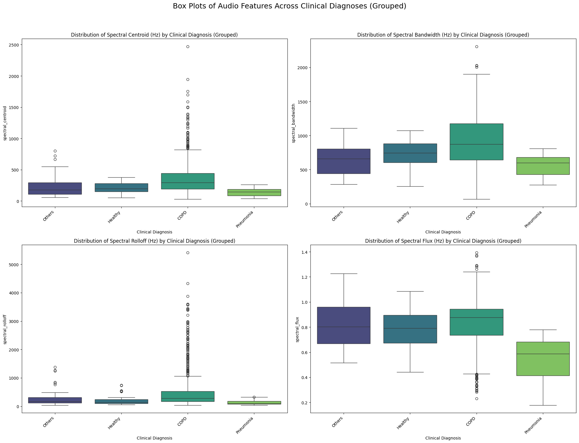
features_to_plot = [
    'spectral_centroid',
    'spectral_bandwidth',
    'spectral_rolloff',
    'spectral_flux'
]

# For display purposes in the title, we can map the internal column names to more readable names
feature_display_names = {
    'spectral_centroid': 'Spectral Centroid (Hz)',
    'spectral_bandwidth': 'Spectral Bandwidth (Hz)',
    'spectral_rolloff': 'Spectral Rolloff (Hz)',
    'spectral_flux': 'Spectral Flux (Hz)'
}

# Create a new 'grouped_diagnosis' column
def group_diagnoses(diagnosis):
    if diagnosis in ['Healthy', 'COPD', 'Pneumonia']:
        return diagnosis
    else:
        return 'Others'

features_df_grouped = features_df.copy()
features_df_grouped['grouped_diagnosis'] = features_df_grouped['clinical_diagnosis'].apply(group_diagnoses)

plt.figure(figsize=(20, 16))

for i, feature_col_name in enumerate(features_to_plot):
    plt.subplot(2, 2, i + 1)  # 2 rows, 2 columns
    sns.boxplot(
        data=features_df_grouped,
        x='grouped_diagnosis', # Use the new grouped diagnosis column
        y=feature_col_name, # Use the actual column name
        palette='viridis'
    )
    plt.title(f'Distribution of {feature_display_names[feature_col_name]} by Clinical Diagnosis (Grouped)') # Use display name in title
    plt.xlabel('Clinical Diagnosis') # Add a clear label for the x-axis
    plt.xticks(rotation=45, ha='right')

plt.suptitle('Box Plots of Audio Features Across Clinical Diagnoses (Grouped)', fontsize=18)
plt.tight_layout(rect=[0, 0.03, 1, 0.95])
plt.show()

/tmp/ipython-input-1969003633.py:30: FutureWarning: 

Passing `palette` without assigning `hue` is deprecated and will be removed in v0.14.0. Assign the `x` variable to `hue` and set `legend=False` for the same effect.

  sns.boxplot(
/tmp/ipython-input-1969003633.py:30: FutureWarning: 

Passing `palette` without assigning `hue` is deprecated and will be removed in v0.14.0. Assign the `x` variable to `hue` and set `legend=False` for the same effect.

  sns.boxplot(
/tmp/ipython-input-1969003633.py:30: FutureWarning: 

Passing `palette` without assigning `hue` is deprecated and will be removed in v0.14.0. Assign the `x` variable to `hue` and set `legend=False` for the same effect.

  sns.boxplot(
/tmp/ipython-input-1969003633.py:30: FutureWarning: 

Passing `palette` without assigning `hue` is deprecated and will be removed in v0.14.0. Assign the `x` variable to `hue` and set `legend=False` for the same effect.

  sns.boxplot(