Laboratory Task 4 – PyTorch Regression#
Name: Joanna Reyda Santos
Section: DS4A
Instruction: Train a linear regression model in PyTorch using a regression dataset. Use the following parameters.
Criterion: MSE Loss
Fully Connected Layers x 2
Batch Size: 8
Optimizer: SGD
Epoch: 1000
# Import necessary libraries
import torch
import torch.nn as nn
import torch.optim as optim
from torch.utils.data import DataLoader, TensorDataset
from sklearn.datasets import make_regression
from sklearn.model_selection import train_test_split
from sklearn.preprocessing import StandardScaler
import matplotlib.pyplot as plt
# Generate a simple regression dataset
X, y = make_regression(n_samples=200, n_features=1, noise=15, random_state=42)

# Scale inputs and outputs for stable training
scaler_X = StandardScaler()
scaler_y = StandardScaler()
X = scaler_X.fit_transform(X)
y = scaler_y.fit_transform(y.reshape(-1, 1))

# Convert to tensors
X = torch.tensor(X, dtype=torch.float32)
y = torch.tensor(y, dtype=torch.float32)

# Split into training and testing sets
X_train, X_test, y_train, y_test = train_test_split(X, y, test_size=0.2, random_state=42)

# Create DataLoader
BATCH_SIZE = 8
train_data = TensorDataset(X_train, y_train)
train_loader = DataLoader(train_data, batch_size=BATCH_SIZE, shuffle=True)
# Two fully connected layers as specified
class LinearRegressor(nn.Module):
    def __init__(self):
        super().__init__()
        self.fc1 = nn.Linear(1, 8)  # input layer → hidden layer
        self.fc2 = nn.Linear(8, 1)  # hidden layer → output layer

    def forward(self, x):
        x = self.fc1(x)
        x = self.fc2(x)
        return x

# Initialize model
model = LinearRegressor()
# Define Loss Function and Optimizer
criterion = nn.MSELoss()                # Mean Squared Error
optimizer = optim.SGD(model.parameters(), lr=0.01)
EPOCHS = 1000
# Training Loop
loss_history = []

for epoch in range(EPOCHS):
    for inputs, targets in train_loader:
        # Forward pass
        preds = model(inputs)
        loss = criterion(preds, targets)

        # Backward pass and optimization
        optimizer.zero_grad()
        loss.backward()
        optimizer.step()

    loss_history.append(loss.item())

    # Display every 100 epochs
    if (epoch + 1) % 100 == 0:
        print(f"Epoch [{epoch+1}/{EPOCHS}] - Loss: {loss.item():.6f}")
Epoch [100/1000] - Loss: 0.034642
Epoch [200/1000] - Loss: 0.030637
Epoch [300/1000] - Loss: 0.040967
Epoch [400/1000] - Loss: 0.009145
Epoch [500/1000] - Loss: 0.030011
Epoch [600/1000] - Loss: 0.068618
Epoch [700/1000] - Loss: 0.040779
Epoch [800/1000] - Loss: 0.047060
Epoch [900/1000] - Loss: 0.062211
Epoch [1000/1000] - Loss: 0.020562
# Evaluate model on test data
model.eval()
with torch.no_grad():
preds = model(X_test)
test_loss = criterion(preds, y_test)
print(f"\nFinal Test MSE Loss: {test_loss.item():.6f}")
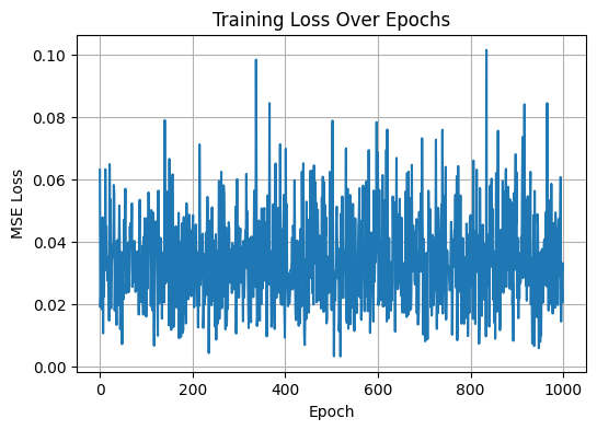
# Plot training loss
plt.figure(figsize=(6,4))
plt.plot(loss_history)
plt.title("Training Loss Over Epochs")
plt.xlabel("Epoch")
plt.ylabel("MSE Loss")
plt.grid(True)
plt.show()
Final Test MSE Loss: 0.036329
# Compare predicted vs. true target values (visual + print)
import matplotlib.pyplot as plt
model.eval()
with torch.no_grad():
sample_inputs, sample_targets = next(iter(train_loader))
predictions = model(sample_inputs)
# Print a few values
print("Sample Predictions:\n", predictions[:8])
print("Actual Targets:\n", sample_targets[:8])
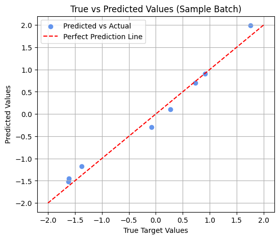
# Visualization
plt.figure(figsize=(6,5))
plt.scatter(sample_targets.numpy(), predictions.numpy(), color='cornflowerblue', label='Predicted vs Actual')
plt.plot([-2, 2], [-2, 2], 'r--', label='Perfect Prediction Line') # reference line
plt.xlabel("True Target Values")
plt.ylabel("Predicted Values")
plt.title("True vs Predicted Values (Sample Batch)")
plt.legend()
plt.grid(True)
plt.show()
Sample Predictions:
 tensor([[-1.4498],
        [ 0.1011],
        [-1.5162],
        [-0.2991],
        [-1.1715],
        [ 0.6983],
        [ 1.9893],
        [ 0.9049]])
Actual Targets:
 tensor([[-1.6125],
        [ 0.2723],
        [-1.6187],
        [-0.0782],
        [-1.3716],
        [ 0.7374],
        [ 1.7588],
        [ 0.9156]])
Reflection#
Based on the results, the model’s loss gradually decreased over 1000 epochs, showing that the regression model successfully learned the relationship between the input and target values. The predicted vs. actual scatter plot also showed that the points aligned closely with the perfect prediction line, indicating good accuracy. This exercise helped me understand how PyTorch automates gradient computation and how adjusting hyperparameters like learning rate can affect model convergence.